How should the PRTools ROC plot be interpreted?

“Roccurves” by BOR at English Wikipedia – Transferred from en.wikipedia to Commons.. Licensed under CC BY-SA 3.0 via Wikimedia Commons

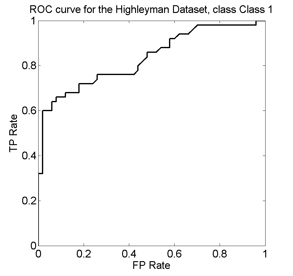
The traditional Receiver-Operator Characteristic (ROC) shows true positive rate (vertically) of a classifier against the false positive rate (horizontally). Wikipedia shows the example on the right for three different decision procedures. By changing the decision threshold these rates change and the curves arise.

These curves can be used in two way. For a desired true positive rate (e.g. the useful yield of some production) they show how this should be paid by the rate of false negatives (e.g. the fraction of useless products). In the other direction one can find what the true positive rate is for a given false negative rate.

In PRTools classifier performances are reported by classification errors. They can be distinguished in errors of the first kind (the classification error in some target class) and errors of the second kind (the classification error of the other class). In order to be consistent within PRTools, its ROC plot shows these two errors against each other.

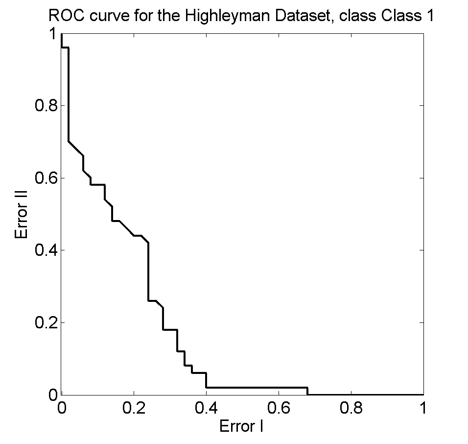
The figure on the left shows the standard PRTools ROC plot. It is based on the following code:

a = gendath;    % generate data
w = a*fisherc;  % compute the Fisher classifier
e = prroc(a,w); % compute ROC plotting data
plote(e);       % plot the curve

The classification error in the target class, Error I, is one minus the true positive rate. The errors in the non-target class, Error II, equals the false positive rate. By the following statements the PRTools ROC plot can be converted into the more standard one on the right:

[e.error e.xvalues e.ylabel e.xlabel] ...
= deal(1-e.xvalues,e.error,'TP Rate','FP Rate');
plote(c);

For more information, see the help file of the prroc routine or the extensive Wikipedia page on the topic.