Kernel-induced space versus the dissimilarity space

The dissimilarity representation has a strong resemblance to a kernel. There are, however, essential differences in assumptions and usage. Here they will be summarized and illustrated by some examples.

Dissimilarities and kernels are both functions describing the pairwise relations between objects. Dissimilarities can be considered as a special type of kernel if kernels are understood as arbitrary functions of two objects (or variables). Very often, especially in the literature on machine learning and pattern recognition over the past 20 years, kernels are related to the kernel trick, enabling the kernelization of various vector space based procedures for data analysis. Here we will use them in that more restricted sense.

The kernel trick relies on the observation that many algorithms defined for Euclidean (or Hilbert) vector spaces can be entirely written in terms of inner products between a given set of vectors:

Here is a function of an arbitrary object optimized for a set of given examples . It can be thought e.g. as a classifier or a mapping to a subspace. gives the same result as , if applied to the same and , but is entirely written in terms of inner products, or . This is possible for classifiers such as the support vector machine or Fisher’s linear discriminant, but also for a linear feature reduction procedure such as the principal component analysis. These procedures can be kernelized.

The great advantage of this is based on the observation that there is a class of kernel functions , operating on the elements of , e.g. the square function or the radial basis function, that result in a new kernel matrix which again can be understood as the Gram matrix in some vector space. Functions that satisfy the Mercer conditions have this property. As a consequence, the same procedure can be used to compute various non-linear versions of , depending on the chosen kernel function :

Like kernels, dissimilarities relate objects pairwise, resulting in a dissimilarity matrix . Now the objects  are not necessarily represented as a feature vector, but they can be, for instance, images, time signals, videos or text files. It just needs to be possible to compute a dissimilarity between any two objects. stands for the set of available objects and  is the Cartesian product, relating any object in with any other object in  or itself.  has thereby the same size as .

In the dissimilarity space approach the dissimilarity matrix is interpreted as a set of vectors representing the original objects as vectors in an Euclidean space. These vectors are defined by pairwise dissimilarities from to all other objects in .  In the dissimilarity space the same procedures may be used for dimension reduction, feature extraction and classification as in any other vector space. The dissimilarity space is thereby an Euclidean space by postulation. The dissimilarity distance , however, can be any proximity function, similarity or dissimilarity, between two objects. It can even by asymmetric or negative for some objects. The most common properties, however, are, that it is non-negative and only zero for identical objects. It is very common in practical applications that it is non-Euclidean and sometimes even non-metric.

While kernels were originally defined between vectors but later extended to other non-vectorial data as well as non-Mercer kernels and non-Euclidean distances, the dissimilarity space approach followed the other direction as researchers wondered about its performance on Euclidean distances derived in the traditional feature space. Functions defined for a vector representation can thereby be applied to dissimilarity data resulting in a non-linear version of the original function (which in this case does not has to be an original linear function):

Consequently, the two approaches meet in two domains: by extending the original kernel approach to non-Mercer kernels and non-vector spaces they meet in almost unrestricted comparison of objects given by raw data. When we apply the dissimilarity approach to Euclidean vector spaces, we operate in the traditional domain of kernels: finding non-linear approaches int he anlysis of vector input spaces.

Below, we will give examples for both cases.

Example 1.

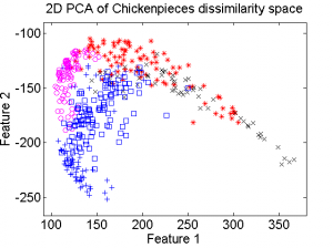
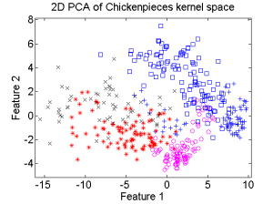
The first example is based on one of the Chickenpieces dissimilarity datasets It is a five class problem given by the dissimilarities between all 446 blob shapes. The scatterplot of the 2D PCA computed in the dissimilarity space is shown on the left plot below. From the dissimilarities a kernel can be computed. As the dissimilarities are non-Euclidean the kernel is non-positive definite (npd) and thereby does not fulfill the Mercer conditions. The right plot shows the 2D PCA of the kernel space is shown. It is clearly visible that there is a non-linear relation between the two spaces.

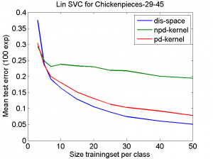
A linear support vector machine classifier (based on the LibSVM package) is computed in the dissimilarity space and based on the derived kernel. As the conditions are not fulfilled, the optimization of the SVM is not guaranteed. A positive definite (pd) version of the kernel has been computed as well. The plot above shows learning curves for these three classifiers. They are based on repeated splits of the dataset in parts for training and testing. In this example the classifier in the dissimilarity space (which can be fully optimized and is based on all information) performs much better than the npd kernel (optimization may fail) or the pd kernel (some information may be lost).

Example 2.

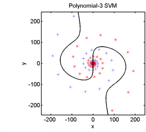
The second example is based on a two-class dataset given in a 2D feature space. It is based on two long spirals. The completel data set is shown in the left plot below. The right plot zooms in on the spiral center.

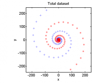
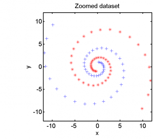
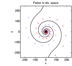
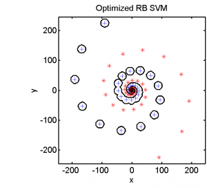
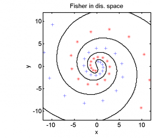
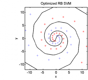
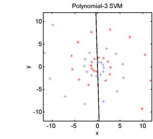
Half of the dataset, systematically sampled, was used for training. On this set we computed a dissimilarity space based on Euclidean distances, the best radial basis function we could find and a polynomial kernel. The result of the Fisher’s Linear Discriminant trained in the dissimilarity space is shown in the feature space in the second plot. The third and the fourth plots show the results of the SVM for the two kernels.

The linear classifier in the dissimilarity space is able to separate the entire spirals in an elegant way. The radial basis kernel almost separates the spirals but does not generalize well. The polynomial kernel is not the right one for this problem.

This example shows a significant advantage of the dissimilarity representation. There is no need for a kernel optimization if a proper dissimilarity measure is used. Dissimilarities have a more explicit meaning than kernels. An expert can use his physical knowledge of the problem to define a dissimilarity measure and check it by the nearest neighbor rule or template matching. They did this as long as automatic pattern recognition has been under study.