Discovered by accident

Some discoveries are made by accident. The wrong road brought a beautiful view. An arbitrary book from the library gave a great, new insight. A procedure was suddenly understood in a discussion with colleagues during a poster session. In a physical experiment a failure in controlling the circumstances showed a surprising phenomenon.

Children playing with simple blocks may discover that a castle or a ship is hidden in the heap. They randomly combine them. A surprising result may suddenly appear, depending on their imagination. When they are sufficiently skilled they may start to beautify it. Perhaps several trials are needed, but then it is there: a beauty.

During one of the lab courses students were investigating some pattern recognition issues using PRTools. It was explained that in some situations the performance of a classifier could be improved by a feature reduction to remove some noise and to run the classifier in a space of lower dimension. The sequence of feature extraction and classifier training can be combined into a single operation. So they compared

classf1 = fisherc;            % straightforward Fisher classifier
classf2 = pcam(0.95)*fisherc; % 95% PCA reduction followed by Fisher


by

testset*(trainset*classf1)*testc
testset*(trainset*classf2)*testc

Note that in PRTools the *-operator is a overloaded by piping: it feeds the data stream from left to right into functions (called mappings) that handle data and can output new data or trained classifiers. The routine testc evaluates the trained classifiers. The examples used in the lab course showed that this is useful for high dimensional data, but not for low dimensional problems, as then PCA may remove useful directions in the feature space. For instance, try the k-dimensional 8-class problem generated by genmdat('gendatm',k,m*ones(1,8))), in which m is the number of training objects per class. One of the students tried by accident:

classf3 = fisherc*fisherc;

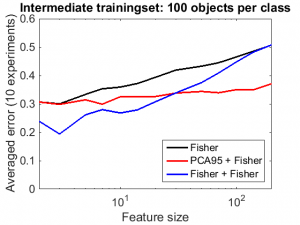
instead of classf2. It appeared that it is also helpful, and was in lower dimensional situations even much more effective than classf2. On the right a feature curve is shown that illustrates this. It is based on an 8-class problem  The entire experiment can be found here. How may the performance of classf3 be explained?

It should be noted that in the above procedures, classf2 and classf3, the same data has been used twice, once for the dimension reduction and once for training the classifier. In classf3 fisherc reduces the dimension of the feature space to 8, the number of class confidences. As these sum to one, the intrinsic dimension is in fact at most 7. This reduction is based on a supervised procedure. For training sets that are sufficiently large in relation with the feature size, this training result is not overtrained and thereby there is room for a second supervised generalization. For large feature sizes, however, the first fisherc is overtrained and the dataset used for training is biased when submitted to the second fisherc. For high dimensional feature spaces (compared with the size of the training set) an unsupervised procedure is needed to enable a useful training procedure based on the same data.

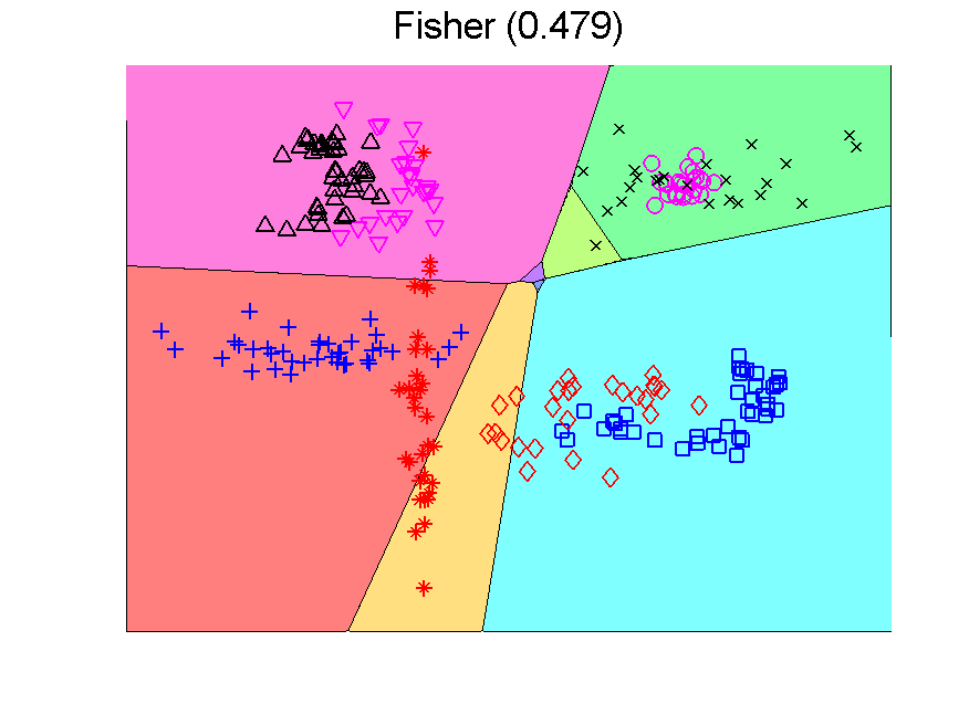
There is a second point to realize. The Fisher classifier is a linear classifier. The separation boundaries between classes are linear. The outputs of the classifier, the class confidences, however, are non-linear functions of the features due to the use of a sigmoid function that transforms distances to classifiers into 0-1 confidences. When these outputs are used as inputs for a second classifier, the overall result of the class boundaries is nonlinear. Below this is illustrated in a two-dimensional problem. The error measured by a large independent test set in given between brackets.

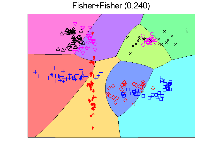
The procedure resulting in the second plot can be understood as generating an 8-dimensional space, because it is an 8-class problem. In this space the Fisher classifier is trained. This yields the observation that any classifier applied to this problem generates such an 8-dimensional space and may in the same way be followed by a second classifier. If the first classifier, producing the space, is not overtrained, more advanced classifiers may be used as the second one. Below some examples are presented using QDA (the PRTools routine qdc).

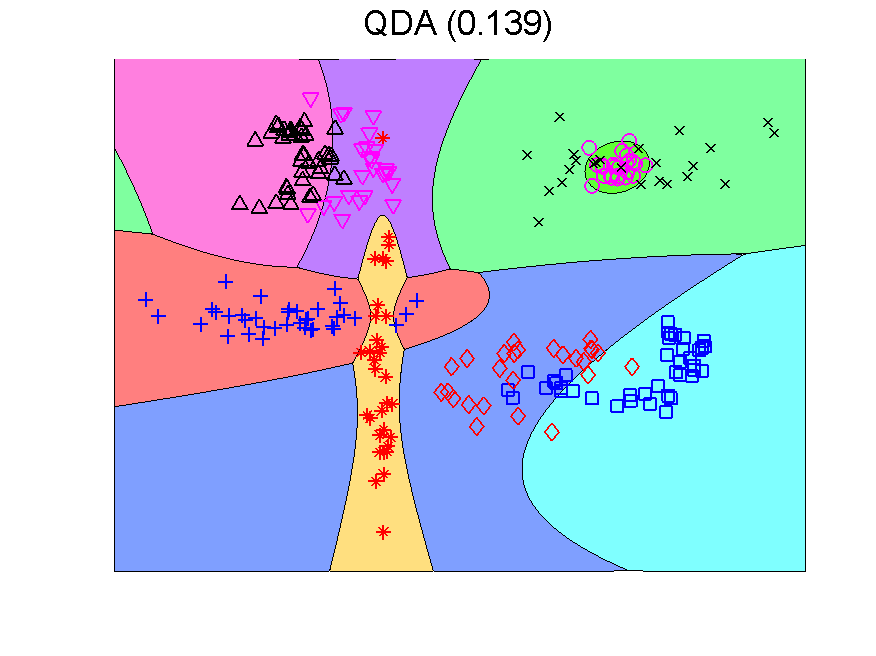
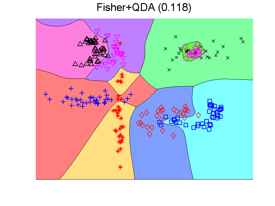
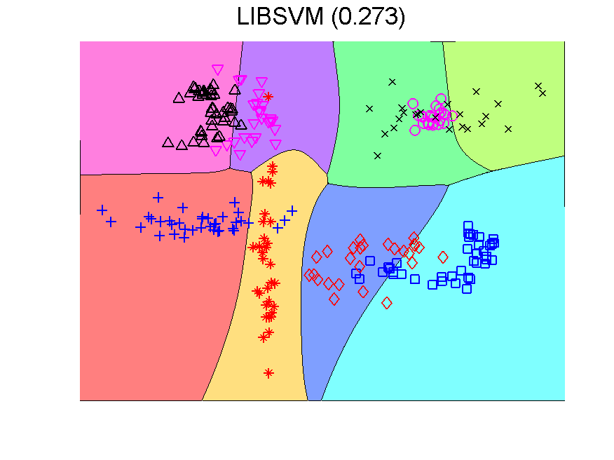
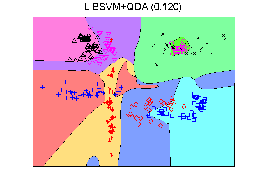
The series starts with just QDA in the original 2-dimensional space. This classifier is improved by first transforming this space to 8-dimensions. The second example shows that the multi-dimensional LIBSVM classifier is non-linear. Apparently it is not overtrained as its outputs can be used to train QDA such that it improves the original classifier. These figure are taken from a more extensive example.

The accidental discovery made by the student is not yet fully exploited. The sequential combination of classifiers in multi-class problems is an interesting area of research.