How should I interpret the output of a classifier?
PRTools distinguishes two types of classifiers: density based and distance based. Some classifiers follow a slightly different concept but are squeezed into these two types.
- Density based classifiers, e.g.
qdc,ldc,udc,mogc,parzenc,naivebc - Distance based classifiers, e.g.
fisherc,svc,loglc - Other ones, e.g.
knnc,lmnc,treec,dtc
Density based classifiers
Density based classifiers estimate for every class a probability density function ![]() in which
in which ![]() is the class and
is the class and ![]() the vector representing an object to be classified. Classification can be done by weighting the densities by the class priors
the vector representing an object to be classified. Classification can be done by weighting the densities by the class priors ![]() :
:
and selecting the class with the highest weighted density:
Sometimes we want to use posterior probabilities (numbers in the ![]() ] interval) instead of weighted densities (
] interval) instead of weighted densities (![]() ). They just differ by normalization:
). They just differ by normalization:
They result into the same class assignments
as the normalization factor ![]() is independent of
is independent of ![]() . Here is a PRTools example based on the classifier qdc which assumes normal densities. The routine classc takes care of normalization;
. Here is a PRTools example based on the classifier qdc which assumes normal densities. The routine classc takes care of normalization;
a = gendatd;       % generate two normal distributions

[test,train] = gendat(a,[2 2]); % 2 test objects per class

w = qdc(train);    % train the classifier

F = test*w;        % weighted densities of the test objects

+F, % show them

0.0005    0.0000

0.0062    0.0004

0.0000    0.0078

0.0000    0.0075

P = test*w*classc;  % compute posterior probabilities

+P, % show them

0.9887    0.0113

0.9415    0.0585

0.0020    0.9980

0.0014    0.9986
After computing F or P the class labels assigned for the test objects can be found by
F*labeld % Generates the same result as for P*labeld

1

1

2

2
Distance based classifiers
Distance based classifiers assign class labels on the basis of distances to objects or separation boundaries. Densities and thereby posterior probabilities are not involved. In order to find a confidence measure comparable to posterior probabilities, PRTools transforms for the distance ![]() to the separation boundary (which are in the interval (
to the separation boundary (which are in the interval (![]() ) by a sigmoid function to the interval (0,1). Distances are scaled before the sigmoid is taken by a maximum-likelihood approach: the likelihood over the training set used for the classifier is optimized. Classifier conditional posteriors are obtained for two classes
) by a sigmoid function to the interval (0,1). Distances are scaled before the sigmoid is taken by a maximum-likelihood approach: the likelihood over the training set used for the classifier is optimized. Classifier conditional posteriors are obtained for two classes ![]() and
and ![]() by using the optimized sigmoid and one minus this sigmoid.
by using the optimized sigmoid and one minus this sigmoid.
See also our paper on this topic (Classifier conditional posterior probabilities, SSSPR 1998, 611-619). This approach is followed for all classifiers that optimize a separation boundary like fisherc, svc and loglc. Multi-class problems are solved in by a one-class-against-rest procedures (mclassc) that results in a confidence for every class.
By applying the inverse sigmoid function invsigm posterior probabilities computed in the above way can be transformed backwardly into distances. It has to be realized, however, that these distance are not the Euclidean distances in the given vector space but that they are scaled in the above way.
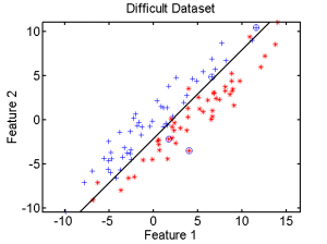
a = gendatd; % generate two normal distributions

[test,train] = gendat(a,[2 2]); % select 2 test objects per class

scatterd(a); % scatterplot of all data

hold on; scatterd(test,'o'); % mark test objects

w = fisherc(a); % compute a classifier

plotc(w); % plot it

d = test*w; % classify test objects

+d % show posteriors

0.8920    0.1080

0.6929    0.3071

0.0220    0.9780

0.0000    1.0000

+(d*invsigm) % show scaled distances

2.1110   -2.1110

0.8137   -0.8137

-3.7946    3.7946

-11.4872   11.4872
Other classifiers
There are various other classifiers that do not fit naturally in the above scheme, e.g. as they compute distances to objects that cannot be negative. Here it is shortly indicated for some of them how they are squeezed in the above concept.
- The one-nearest-neighbor classifier
knnc([],1) - All other nearest neighbor classifiers estimate directly posteriors by the counting the numbers of objects
 for all
  classes in a neighborhood of
  objects. Bayes estimators are used:
  .
. - The nearest mean classifier
nmcuses postulated spherical Gaussian densities around the means and computes posteriors from that assuming that all classes have the same prior. - The scaled nearest mean classifier
nmscis a density based classifier that assumes spherical Gaussian densities after scaling the axes. It is thereby equivalent toudc. - Neural network classifiers like
lmnc,bpxnc,rbncandrnncuse the normalized outputs as posteriors. - Decision trees such as
treecanddtcuse the same Bayes estimators likeknncover the number of training objects found in their end nodes.

