How can PRTools be used for studying the dissimilarity representation?

Many studies have been presented on the dissimilarity representation in which experiments are based on PRTools. A large collection of research tools has thereby been developed. As research in this direction is still in progress by various researchers, a stable and consistent toolbox is not yet ready. There are however many possibilities to develop and run dissimilarity based experiments directly on PRTools. Here follows a very short introduction.

Obtaining or constructing a dissimilarity matrix

• Existing artificial and real world datasets can be downloaded by the prdisdataset package.
• The PRTools routines proxm and distm may be used to compute dissimilarity matrices from feature based representation given by a PRTools dataset.
• Raw data (images, spectra, time signals) given by a PRTools datafile may serve as input for a user supplied routine to compute dissimilarities between such objects.

A dissimilarity matrix should be supplied as an ordinary, labeled PRTools dataset with as many columns as rows. The columns refer to the same objects as the rows. For some routines it is needed that the PRtools feature names labeling these colums are identical to the corresponding object labels assigned to the rows. This might be done by a call like:

a = setfeatlab(a,getlabels(a))

Classifiers in dissimilarity space

A dissimilarity matrix, given by a dataset as described above, can be interpreted as a feature matrix. It is a set of objects represented as vectors(dissimilarities to other objects)  in a vector space, the dissimilarity space. Procedures for feature spaces apply here is well. The original dimensionality of the dissimilarity space is equal to the number of objects. Dimension reduction may thereby be needed for some classifiers. In contrast to feature spaces random selection of e representation set is a sensible procedure here, next to other procedures for feature and prototype selection. An example:

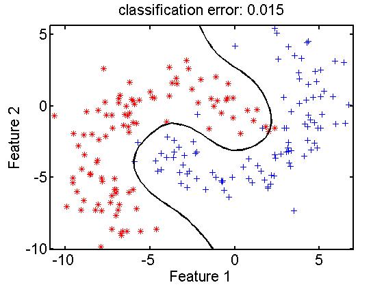
data= gendatb([200,200]);              % raw data in 2D feature space
[trainset,testset] = gendat(data,0.5); % 50-50 split in train and testset
repset = gendat(trainset,0.25);        % random 25% for representation
disspace = proxm(repset,'d',1);        % map to dis space by eucl. dist.
trainrep = trainset*disspace;          % map the trainset into dis space
classf = trainrep*ldc;                 % compute a classifier by ldc
e = testset*disspace*classf*testc;     % map testset, classify and test
scatterd(trainset);                    % show original feature space
plotc(disspace*classf);                % show classifier in this space
title(['classification error: ' num2str(e,'%5.3f')]); % error in title

Note that the classifier in the dissimilarity space is a linear one (ldc). It shows as a non-linear classifier in the original feature space due to the non-linear relation between these spaces: the Euclidean distance measure.

This example is, for simplicity, based on a feature space. It results there in an interesting, good performing classification function. PRTools offers an integrated classifier, fdcs. In contrast to the support vector classifier there is no need for kernel optimization as the dissimilarity measure does this in a natural way. See a paper on this topic for more information.

In case of given dissimilarities the above example simplifies as the computation and application of the mapping to the dissimilarity space (disspace in the example) is not needed.

Embedding

The dissimilarity space as used above is a postulated euclidean space using the dissimilarities to the representation set as axes. There are no formal restriction w.r.t. the dissimilarity measure. If dissimilarities are positive, symmetric, and zero between an object and itself it might be possible to construct a set of vectors in an euclidean space in such a way that their distances are identical to the given ones. In order to obtain a proper euclidean space the given dissimilarities have to be euclidean as well. Otherwise a so-called Pseudo-Euclidean space (PE-space) has to be constructed. PRTools has no tools to construct such a PE-space, but an approximate euclidean space can always be found using the tools for MultiDimensional Scaling (MDS, implemented by mds). This is a non-linear mapping. A linear mapping can be found by so-called classical scaling, implemented by mds_cs.

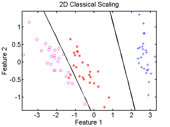
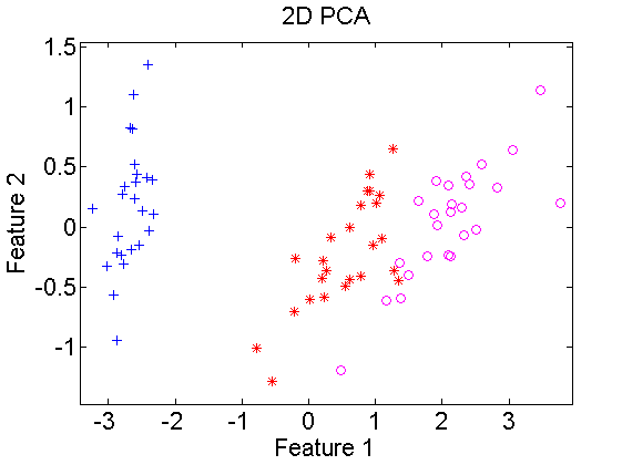
In the below example first euclidean distances are computed for the Iris dataset, which is 4-dimensional. It is split in sets for training and testing.  Using classical scaling a 2-dimensional embedding is found for the training set and a 2-dimensional classifier is computed. The classifier is projected in the embedded space and classified. In the right figure for comparison a 2-dimensional PCA is computed. This shows that the result, apart from rotations and translations, is very similar to classical scaling.

data = iris;                      % load dataset, prdatasets in path
dismap = proxm(data,'d',1);       % define dissimilarity mapping
% to training set
emmap = data*dismap*mds_cs([],2); % map training, compute 2D embedding mapping
classf = data*dismap*emmap*qdc;   % map training set by both mappings
% and compute classifier
scatterd(data*dismap*emmap);      % plot scatter
plotc(classf)                     % plot classifier
title('2D Classification Scaling');
figure;
scatterd(data*pcam(trainset,2));  % plot pca scatter
title('2D PCA')