Peaking summarized

Pattern recognition learns from examples. Thereby, generalization is needed. This can only be done if the objects, or at least the differences between pattern classes have a finite complexity. That is what peaking teaches us. We will go once more through the steps. (See also our previous discussions on peaking, dimensionality problems and Hughes’ phenomenon).

The basic cause of peaking

If the set of given examples is as large as the universe the problem is just computational. For the recognition of a new object we have to find it in the given set. If the objects have an infinite complexity this may not be possible in finite time, unless the pattern class differences are finite. Learning has to determine this.

If the given set is smaller, a new object may be different from any given object. Now the problem is fundamental. The set of examples has to be generalized such that new, never observed objects can be recognized. Is this possible if the complexity of class differences is larger than the set of examples? In that case not all differences can be covered. We have more unknowns (class differences)  than conditions (examples).

This sketches the problem underlying the peaking phenomenon: when it really happens, when it happens in expectation and when it happens on average over a set of problems.

The basic phenomenon

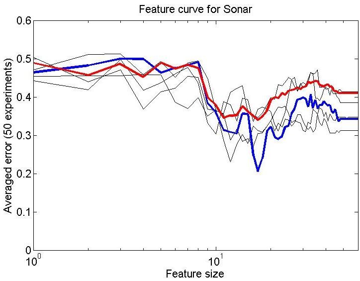
Let us take a real world 2-class dataset, e.g. the classical sonar dataset (class sizes 111 and 97) and split it in a training set of 10 objects per class and a test set constituted by the remaining objects. As a classifier we use the 1-NN rule. The error as a function of the number of features is shown in the left figure for various splits. The blue line shows the average over 50 repetitions.

There is a clear peaking observable for about 15 features. After that the error increases. The individual curves show a high variability due to the random dataset splits. Even the average curve looks noisy. This is due to the different characteristics of the features.

We are only able to compute these curves as we have a larger dataset that enables us to separate out a test set. In practice this will not be the case. So, let us assume that we have just a dataset of 20 objects, 10 per class. Now, a leave-one-out error estimate may be used: 10+9 objects are used for training the classifier and the remaining, excluded object is tested. This is rotated over all objects. The result, the red curve, is slightly worse (as the test object is always from the minority class), but the peaking is still observable. So this procedure may be used to find the optimal feature size. (It is used in the feateval PRTools routine for feature evaluation; the ‘NN’ criterion).

Features may be given in an order raging from important to unimportant. In many real applications this is unknown. If it is known, however, it may be better to give a smaller weight to the higher ranked features. How to do this is unclear, as this has to be done before the training. Also evaluation is not straightforward. If it could have been evaluated this might have been used for optimizing the weights. By that the weight design would be included in the training. But … we tried to set the weights before the training.

If the feature ranking is arbitrary the way to proceed is to rank them according to some feature evaluation or by a feature selection procedure. The latter is only possible with a sufficient accuracy if the size of the feature set is already sufficiently small given the size of the training set. So for large feature sets one has to start with an individual feature evaluation.

In all these procedures there is always the danger that some weak features perform seemingly well due to noise and are selected. If later an additional labeled dataset becomes available it might become clear that such features are used but in fact perform bad and are the cause of peaking. In conclusion, in real applications peaking cannot entirely, with certainty, be avoided.

The expected classification error

In many studies on the peaking phenomenon one takes a particular problem and studies the expected error. The expectation is over the selection of the training set. The red and blue curves in the figure above are the averages of 50 experiments in which each time a new training set is selected. This approximates the expected error. It can only be studied for artificial problems or situations as one needs the possibility to generate new training sets. In a real application just one of them will be available. If one would combine them into a single, larger training set this set is expected to generate a better classifier. The possibility of a good evaluation by an independent test set, however, is thereby destroyed.

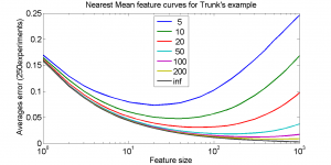
Studies on the expected classification error, like Trunk’s example, just show what might happen. They are thereby theoretical studies on the peaking phenomenon. They may result in a sensitivity of various classifiers for peaking in particular problems. Thereby knowledge is gained on classification procedures in relation to problem characteristics. They are not directly a tool to avoid peaking in a given application.

The mean classification error

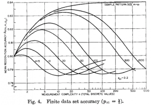
How sensitive is a particular classification procedure for peaking? In order to answer this question one has to define a set of problems and study an average of the resulting expected classification errors. An example is the study by Hughes. As was pointed out by Van Campenhout, his study was inconsistent as the considered set of problems was not constant over the problem complexities.

The result of such a study, if performed well, may be that one may find for every problem complexity (feature size) the classifier that performs best in expectation over the set of problems. Such a result may be valuable for application areas in which the set of problems is reasonably well defined but in which frequently new classifiers have to be designed.

An example is the classification of speakers in a recorded discussion on the basis of a small audio training set. The best classifier, on average, will depend on the size of this training set. This classifier has to use an optimized feature set for the selected training size taking into account the peaking phenomenon. It is possible to determine the classifier and the feature set on the basis of a representative set of recorded discussions as a function of the training set size.

Finally

Peaking, or overtraining exists and occurs frequently. Balancing feature size, training set size and the choice of the classifier is a basic problem in the design of pattern recognition systems. The inclusion of an additional, noisy and not very informative feature can always destroy the performance. By accident such features may look well. If one considers many candidates the probability that such a feature is encountered becomes high. Consequently, some knowledge should be available to avoid this.