Trunk’s example of the peaking phenomenon

In 1979 G.V. Trunk published a very clear and simple example of the peaking phenomenon. It has been cited many times to explain the existence of peaking. Here, we will summarize and discuss it for those who want to have a better idea about the peaking problem. The paper presents an extreme example. Its value for the pattern recognition practice is thereby mainly to point out the dangers of a careless use of the traditional procedures.

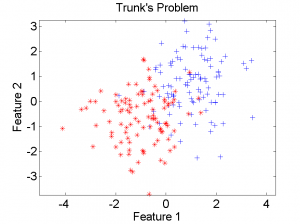
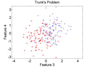
Imagine a two-class problem of normally distributed data. The features are independent and all have a unit variance for both classes. The class means are given by and for feature . (In PRTools this data can be generated by gentrunk). In the two scatter-plots a data set of 100 objects per class is shown for the features no. 1 and 2 (left), and the features no. 3 and 4 (right). Every feature higher in the list has a low class separability, but there is always some contribution, albeit very small asymptotically.

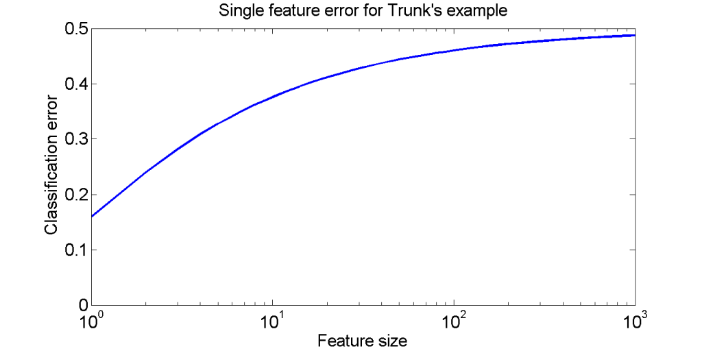
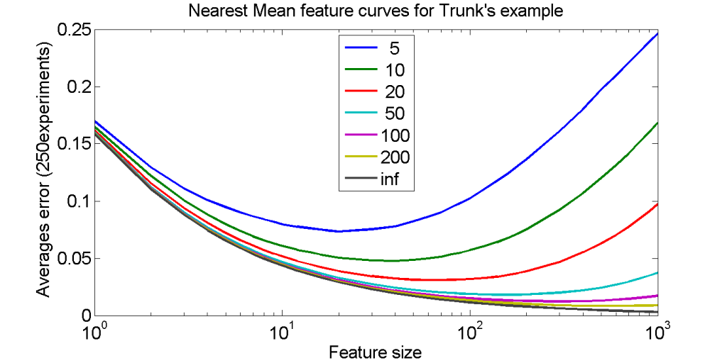
So, the class separability decreases monotonically for increasing number of feature. The class overlap of the individual features is shown in the left figure above.The figure on the right shows the cumulative class overlap for increasing feature sizes, by the bottom black line. Click on the figure for a better look.

The other curves represent the classification error of the nearest mean classifier based on training sets of various sizes. In spite of the fact that features with higher numbers still add to the class separability, their contribution to the total separability becomes so small that the noise introduced by the finite training sets starts to dominate. The result is the peaking phenomenon: more features are counterproductive.

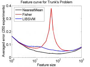
Let us now consider the feature curves for different classifiers and for 25 objects per class only.  The figure on the left shows the classification errors for the Nearest Mean Classifier (nmc in PRTools), Fisher’s Linear Discriminant (fisherc in PRTools) and the linear Support Vector Machine offered by the LIBSVM package (may be called by libsvc from PRTools).

Nearest Mean is by far the simplest classifier but beats the other two everywhere. That is because the mean vectors are the only parameters in which the two classes differ and the distributions of all features are, except for the means, identical. The Fisher discriminant for instance depends on correlations and variance differences. They are not in the problem, but may show up in a finite data set, thereby deteriorating the classification result.

The very remarkable peak in the Fisher curve is located exactly at 50 features, the point where there are as many objects as features. We may discuss this in detail later. Readers who cannot wait may have a look at a paper by Marina Skurichina.

Although the SVM is generally recognized as a very good classifier, it is beaten here by the Nearest Mean classifier. This is for the same reason as holds for the Fisher discriminant. The classifier is much more powerful than needed.

The main point of the example is that all classifiers show the peaking phenomenon: eventually features are added that are almost just noise. Their contribution to the class separability is very small and can only be used if the training set is sufficiently large. For a finite training set there is always a point in which the noise become larger than the separability increase caused by the new feature.

This example shows clearly that datasets can be constructed that show peaking. But…is it realistic? Does it prove that peaking is unavoidable in practical applications?

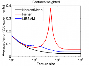
Peaking is here caused by adding new independent features, having the same class variances but smaller and smaller mean differences. What will not happen in practice is that a practitioner knows the ranking of the features but discards it. For instance, if he applies a heavy weighting of features by shrinking the variance of the higher ranked features the error curves may look as shown the right figure: peaking disappears and the asymptotic results are better because  the noisy features carry a very small weight.

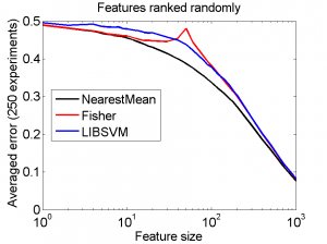
Knowing the exact order of the features w.r.t. their class separability is very uncommon. Also an optimal weighting scheme cannot be derived without additional samples. More realistic is that features are given in some random order. The next figures show the related error curves.

The figure on the left presents the averaged results of a random ranking of the first 1000 features. There is a high probability that one of the many weak features is selected first, but at some moment the better ones will be found. When all features are used the same result will be found as obtained by the original ranking, as classifiers do not depend on the order of the features. Peaking is gone now, but also the better results obtained above before peaking started to strike.

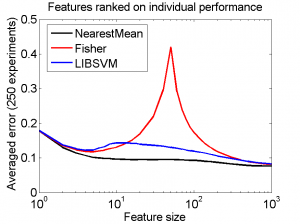
Another, more realistic approach is to rank the features according to their individual performance as measured by the given data, the figure on the right. Asymptotic results are again the same, but good results are found much sooner. Some wiggling can be observed, but the systematic, peaking phenomenon as in the original example is gone.

The conclusion can be drawn that a sharp peaking phenomenon can be constructed but in practice this phenomenon may be much weaker. There are no classifiers that can fully prevent it as it may always happen that a weak feature looks accidentally good in a single dataset and thereby receives a high weight or passes the threshold selection.